The Abacus Bar Code

Imagine you are a gambler. Only imagine mind, in the interests of this thought experiment. Don’t actually do it. It’s not a good idea.

Imagine too that you want to gamble on the horses, and to keep things simple you will just put a small bet, say £1 to win on the favourite of every flat race in the UK (that’s about 5,000 races a year). The first thing you notice is that you don’t make a profit, and the reason for this is straightforward. Bookmakers set the odds for races so that they can top-slice a profit, usually around 15%. This means that if you put £1 on 5,000 races in a year, you would spend £5,000 and get about £4,250 back, hardly satisfactory.

The only way to get around this is to avoid betting on races that are likely to give you the least return and concentrate on those that are likely to give you the best return. It’s a bit like picking the best stocks and shares to buy. But how do you try to make that distinction?

Horse racing is like the weather, in that it has a large number of variables, making it difficult to make predictions. Variables interact and the more variables there are the more complex those interactions. The variables in horse racing include the number of horses, the distance, the odds, the historical performance of both horse and rider, the weather, the condition of the ground and many more. In order to study these variables we would need to have at our back a large number of historical racing results that include information about the variables. Ten years worth would give us data on 50,000 races. A good and simple start is to look at just one variable; lets say the number of horses.

Investment return using the single variable of the number of horses in the race. Source - Me

Again to keep things simple we assume that there are only 10 variations of horse numbers, from 5 - 14. There’s more than that, but as this is a thought experiment, it doesn’t matter. On average each one of the 10 will have 5,000 historical race results to give a return figure we can plot on the graph opposite. If the number of horses in a race has no impact at all on the rate of return, the red line on the graph will match the dotted 85p line. If it does have an impact, the red line will show that impact with roughly equal amounts above and below the dotted line. The part of the curve above the line shows a higher return than 85p, but is still well below the £1 target.

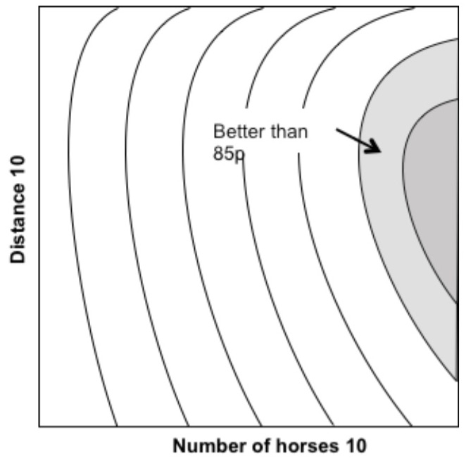
Investment return using two variables (number of horses and race distance). Source - Me

So now we need to introduce a second variable, say the distance of the race. This time we can’t present this as a graph. To show the relationship between two variables we need what is effectively a contour map (see below). A hill or plateau represents a better return than 85p and a valley or low lying area represents a smaller return than 85p. If we repeat the division of the new variable into ten groups, say from 5 to 14 furlongs, we now have a contour map containing 10 by 10 (100) locations to distribute our 50,000 historical race results. This means that on average each location will have about 500 historical results contributing to its vertical position. This gives a margin of error of ±5%. Not too bad but a lot less than the ±2% achieved with only one variable and 5,000 results per location. We are a little bit closer to the £1 target, but still well short.

Any position in this onion can be defined by three coordinates, Source - Pixabay

So now we need to add a third variable, say the odds of the favourite. This time we can only visualise the three way relationship with a three dimensional object. It can be thought of as the distorted layers of an onion where each layer represents a specific return on investment. Once again we have made a little progress towards £1, but still not enough. Even worse we now have 10 cubed (1,000) locations for our 50,000 historical results which is only 50 per location. The margion of error now is ±14% and therefore we will have much less confidence in the results.

Adding a fourth variable has two dreadful effects. First we can no longer visualise the result, and have to rely on mathematical expression. Second we now have 10 quadrupled (10,000) locations, with only 5 results per location. Accuracy is now completely out the window and we still haven’t got to £1.

You might think that we should give up at this point, but not so. What makes this method useless is the increase in power with the addition of the each new variable (10, then 10 squared, then cubed and so on). What we need is method that doesn’t do this.

That method is multiple regression analysis.

Multiple regression analysis is not so much mathematically complex as mathematically tedious and time consuming. For this reason the only way it can be done is by a computer doing the tedious bits, and delivering outcomes. Choosing a model to illustrate the principle without using too much maths has been an interesting exercise. This is the result and it should become clear why I have called it the abacus bar code model.

Imagine an abacus with only one bead on each wire (above). Each wire represents a variable, and is scaled accordingly (number, distance, odds etc). The single beads mark out a distinctive track across the variables. Its a kind of barcode for the future race we are attempting to assess. Once the track of the future race is in place, the track of each of the 50,000 historical races is individually compared to the target track. A numerical value is calculated that defines the difference between the two tracks. If the difference is small (close) the historical result is given a strong mathematical influence on the predicted return. If it large (far away) it is given a correspondingly weak influence. Others are either somewhere in between or a mixture (all over the place).

The Abacus Barcode model for multiple regression analysis. Source - Me

The final predicted return for the future race is an aggregate of all the 50,000 influences. The calculations also provide a second piece of information, called a T value. This delivers a numerical assessment of the significance of each variable to the final prediction. It is then possible to remove the least significant variables one by one, re-running the programme each time until the accuracy of the prediction is maximised.

And that, ladies and gentleman, is multiple regression analysis, Its defining characteristic being that all the variables can be used without weakening confidence because margins of error are kept within reasonable limits.

A cautionary note

This is just a thought experiment to describe regression without using too much maths. There’s no guarantee that it would even work for horse racing.

Just in case you were thinking of giving this a go anyway, I should warn you that it’s not even practical. The odds of the favourite in this scenario are not finalised until the few seconds before a race starts. The odds are a significant contributer to the calculations and there would be no time to run a regression programme in those few seconds.

So don’t try it